4. Circulant Matrices#

4.1. Overview#

This lecture describes circulant matrices and some of their properties.

Circulant matrices have a special structure that connects them to useful concepts including

convolution
Fourier transforms
permutation matrices

Because of these connections, circulant matrices are widely used in machine learning, for example, in image processing.

We begin by importing some Python packages

import numpy as np
from numba import jit
import matplotlib.pyplot as plt

np.set_printoptions(precision=3, suppress=True)

4.2. Constructing a Circulant Matrix#

To construct an $N \times N$ circulant matrix, we need only the first row, say,

[\begin{matrix} c_{0} & c_{1} & c_{2} & c_{3} & c_{4} & \dots & c_{N - 1} \end{matrix}] .

After setting entries in the first row, the remaining rows of a circulant matrix are determined as follows:

(4.1)#

\begin{array}{r} C = [\begin{array}{ccccccc} c_{0} & c_{1} & c_{2} & c_{3} & c_{4} & \dots & c_{N - 1} \\ c_{N - 1} & c_{0} & c_{1} & c_{2} & c_{3} & \dots & c_{N - 2} \\ c_{N - 2} & c_{N - 1} & c_{0} & c_{1} & c_{2} & \dots & c_{N - 3} \\ ⋮ & ⋮ & ⋮ & ⋮ & ⋮ & ⋮ & ⋮ \\ c_{3} & c_{4} & c_{5} & c_{6} & c_{7} & \dots & c_{2} \\ c_{2} & c_{3} & c_{4} & c_{5} & c_{6} & \dots & c_{1} \\ c_{1} & c_{2} & c_{3} & c_{4} & c_{5} & \dots & c_{0} \end{array}] \end{array}

It is also possible to construct a circulant matrix by creating the transpose of the above matrix, in which case only the first column needs to be specified.

Let’s write some Python code to generate a circulant matrix.

@jit
def construct_cirlulant(row):

    N = row.size

    C = np.empty((N, N))

    for i in range(N):

        C[i, i:] = row[:N-i]
        C[i, :i] = row[N-i:]

    return C

# a simple case when N = 3
construct_cirlulant(np.array([1., 2., 3.]))

array([[1., 2., 3.],
       [3., 1., 2.],
       [2., 3., 1.]])

4.2.1. Some Properties of Circulant Matrices#

Here are some useful properties:

Suppose that $A$ and $B$ are both circulant matrices. Then it can be verified that

The transpose of a circulant matrix is a circulant matrix.
$A + B$ is a circulant matrix
$A B$ is a circulant matrix
$A B = B A$

Now consider a circulant matrix with first row

c = [\begin{matrix} c_{0} & c_{1} & \dots & c_{N - 1} \end{matrix}]

and consider a vector

a = [\begin{matrix} a_{0} & a_{1} & \dots & a_{N - 1} \end{matrix}]

The convolution of vectors $c$ and $a$ is defined as the vector $b = c * a$ with components

(4.2)#

b_{k} = \sum_{i = 0}^{n - 1} c_{k - i} a_{i}

We use $*$ to denote convolution via the calculation described in equation (4.2).

It can be verified that the vector $b$ satisfies

b = C^{T} a

where $C^{T}$ is the transpose of the circulant matrix defined in equation (4.1).

4.3. Connection to Permutation Matrix#

A good way to construct a circulant matrix is to use a permutation matrix.

Before defining a permutation matrix, we’ll define a permutation.

A permutation of a set of the set of non-negative integers ${0, 1, 2, \dots}$ is a one-to-one mapping of the set into itself.

A permutation of a set ${1, 2, \dots, n}$ rearranges the $n$ integers in the set.

A permutation matrix is obtained by permuting the rows of an $n \times n$ identity matrix according to a permutation of the numbers $1$ to $n$ .

Thus, every row and every column contain precisely a single $1$ with $0$ everywhere else.

Every permutation corresponds to a unique permutation matrix.

For example, the $N \times N$ matrix

(4.3)#

\begin{array}{r} P = [\begin{array}{cccccc} 0 & 1 & 0 & 0 & \dots & 0 \\ 0 & 0 & 1 & 0 & \dots & 0 \\ 0 & 0 & 0 & 1 & \dots & 0 \\ ⋮ & ⋮ & ⋮ & ⋮ & ⋮ & ⋮ \\ 0 & 0 & 0 & 0 & \dots & 1 \\ 1 & 0 & 0 & 0 & \dots & 0 \end{array}] \end{array}

serves as a cyclic shift operator that, when applied to an $N \times 1$ vector $h$ , shifts entries in rows $2$ through $N$ up one row and shifts the entry in row $1$ to row $N$ .

Eigenvalues of the cyclic shift permutation matrix $P$ defined in equation (4.3) can be computed by constructing

\begin{array}{r} P - λ I = [\begin{array}{cccccc} - λ & 1 & 0 & 0 & \dots & 0 \\ 0 & - λ & 1 & 0 & \dots & 0 \\ 0 & 0 & - λ & 1 & \dots & 0 \\ ⋮ & ⋮ & ⋮ & ⋮ & ⋮ & ⋮ \\ 0 & 0 & 0 & 0 & \dots & 1 \\ 1 & 0 & 0 & 0 & \dots & - λ \end{array}] \end{array}

and solving

det (P - λ I) = (- 1)^{N} λ^{N} - 1 = 0

Eigenvalues $λ_{i}$ can be complex.

Magnitudes $∣ λ_{i} ∣$ of these eigenvalues $λ_{i}$ all equal $1$ .

Thus, singular values of the permutation matrix $P$ defined in equation (4.3) all equal $1$ .

It can be verified that permutation matrices are orthogonal matrices:

P P^{'} = I

4.4. Examples with Python#

Let’s write some Python code to illustrate these ideas.

@jit
def construct_P(N):

    P = np.zeros((N, N))

    for i in range(N-1):
        P[i, i+1] = 1
    P[-1, 0] = 1

    return P

P4 = construct_P(4)
P4

array([[0., 1., 0., 0.],
       [0., 0., 1., 0.],
       [0., 0., 0., 1.],
       [1., 0., 0., 0.]])

# compute the eigenvalues and eigenvectors
𝜆, Q = np.linalg.eig(P4)

for i in range(4):
    print(f'𝜆{i} = {𝜆[i]:.1f} \nvec{i} = {Q[i, :]}\n')

𝜆0 = -1.0+0.0j 
vec0 = [-0.5+0.j   0. +0.5j  0. -0.5j -0.5+0.j ]

𝜆1 = 0.0+1.0j 
vec1 = [ 0.5+0.j -0.5+0.j -0.5-0.j -0.5+0.j]

𝜆2 = 0.0-1.0j 
vec2 = [-0.5+0.j   0. -0.5j  0. +0.5j -0.5+0.j ]

𝜆3 = 1.0+0.0j 
vec3 = [ 0.5+0.j  0.5-0.j  0.5+0.j -0.5+0.j]

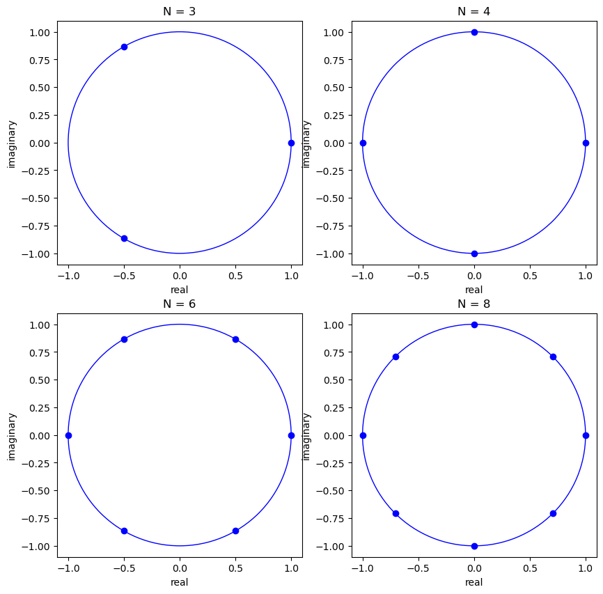
In graphs below, we shall portray eigenvalues of a shift permutation matrix in the complex plane.

These eigenvalues are uniformly distributed along the unit circle.

They are the $n$ roots of unity, meaning they are the $n$ numbers $z$ that solve $z^{n} = 1$ , where $z$ is a complex number.

In particular, the $n$ roots of unity are

z = \exp (\frac{2 π j k}{N}), k = 0, \dots, N - 1

where $j$ denotes the purely imaginary unit number.

fig, ax = plt.subplots(2, 2, figsize=(10, 10))

for i, N in enumerate([3, 4, 6, 8]):

    row_i = i // 2
    col_i = i % 2

    P = construct_P(N)
    𝜆, Q = np.linalg.eig(P)

    circ = plt.Circle((0, 0), radius=1, edgecolor='b', facecolor='None')
    ax[row_i, col_i].add_patch(circ)

    for j in range(N):
        ax[row_i, col_i].scatter(𝜆[j].real, 𝜆[j].imag, c='b')

    ax[row_i, col_i].set_title(f'N = {N}')
    ax[row_i, col_i].set_xlabel('real')
    ax[row_i, col_i].set_ylabel('imaginary')

plt.show()

_images/271af94c1fcb323aec2c765f69d8d2d87e60821fd43536e74b10b22ab4971769.png

For a vector of coefficients ${c_{i}}_{i = 0}^{n - 1}$ , eigenvectors of $P$ are also eigenvectors of

C = c_{0} I + c_{1} P + c_{2} P^{2} + \dots + c_{N - 1} P^{N - 1} .

Consider an example in which $N = 8$ and let $w = e^{- 2 π j / N}$ .

It can be verified that the matrix $F_{8}$ of eigenvectors of $P_{8}$ is

\begin{array}{r} F_{8} = [\begin{array}{ccccc} 1 & 1 & 1 & \dots & 1 \\ 1 & w & w^{2} & \dots & w^{7} \\ 1 & w^{2} & w^{4} & \dots & w^{14} \\ 1 & w^{3} & w^{6} & \dots & w^{21} \\ 1 & w^{4} & w^{8} & \dots & w^{28} \\ 1 & w^{5} & w^{10} & \dots & w^{35} \\ 1 & w^{6} & w^{12} & \dots & w^{42} \\ 1 & w^{7} & w^{14} & \dots & w^{49} \end{array}] \end{array}

The matrix $F_{8}$ defines a Discete Fourier Transform.

To convert it into an orthogonal eigenvector matrix, we can simply normalize it by dividing every entry by $\sqrt{8}$ .

stare at the first column of $F_{8}$ above to convince yourself of this fact

The eigenvalues corresponding to each eigenvector are ${w^{j}}_{j = 0}^{7}$ in order.

def construct_F(N):

    w = np.e ** (-complex(0, 2*np.pi/N))

    F = np.ones((N, N), dtype=complex)
    for i in range(1, N):
        F[i, 1:] = w ** (i * np.arange(1, N))

    return F, w

F8, w = construct_F(8)

(0.7071067811865476-0.7071067811865475j)

F8

array([[ 1.   +0.j   ,  1.   +0.j   ,  1.   +0.j   ,  1.   +0.j   ,
         1.   +0.j   ,  1.   +0.j   ,  1.   +0.j   ,  1.   +0.j   ],
       [ 1.   +0.j   ,  0.707-0.707j,  0.   -1.j   , -0.707-0.707j,
        -1.   -0.j   , -0.707+0.707j, -0.   +1.j   ,  0.707+0.707j],
       [ 1.   +0.j   ,  0.   -1.j   , -1.   -0.j   , -0.   +1.j   ,
         1.   +0.j   ,  0.   -1.j   , -1.   -0.j   , -0.   +1.j   ],
       [ 1.   +0.j   , -0.707-0.707j, -0.   +1.j   ,  0.707-0.707j,
        -1.   -0.j   ,  0.707+0.707j,  0.   -1.j   , -0.707+0.707j],
       [ 1.   +0.j   , -1.   -0.j   ,  1.   +0.j   , -1.   -0.j   ,
         1.   +0.j   , -1.   -0.j   ,  1.   +0.j   , -1.   -0.j   ],
       [ 1.   +0.j   , -0.707+0.707j,  0.   -1.j   ,  0.707+0.707j,
        -1.   -0.j   ,  0.707-0.707j, -0.   +1.j   , -0.707-0.707j],
       [ 1.   +0.j   , -0.   +1.j   , -1.   -0.j   ,  0.   -1.j   ,
         1.   +0.j   , -0.   +1.j   , -1.   -0.j   ,  0.   -1.j   ],
       [ 1.   +0.j   ,  0.707+0.707j, -0.   +1.j   , -0.707+0.707j,
        -1.   -0.j   , -0.707-0.707j,  0.   -1.j   ,  0.707-0.707j]])

# normalize
Q8 = F8 / np.sqrt(8)

# verify the orthogonality (unitarity)
Q8 @ np.conjugate(Q8)

array([[ 1.+0.j, -0.+0.j, -0.+0.j, -0.+0.j, -0.+0.j,  0.+0.j,  0.+0.j,
         0.+0.j],
       [-0.-0.j,  1.+0.j, -0.+0.j, -0.+0.j, -0.+0.j, -0.+0.j,  0.+0.j,
         0.+0.j],
       [-0.-0.j, -0.-0.j,  1.+0.j, -0.+0.j, -0.+0.j, -0.+0.j,  0.+0.j,
         0.+0.j],
       [-0.-0.j, -0.-0.j, -0.-0.j,  1.+0.j, -0.+0.j, -0.+0.j, -0.+0.j,
        -0.+0.j],
       [-0.-0.j, -0.-0.j, -0.-0.j, -0.-0.j,  1.+0.j, -0.+0.j, -0.+0.j,
        -0.+0.j],
       [ 0.-0.j, -0.-0.j, -0.-0.j, -0.-0.j, -0.-0.j,  1.+0.j, -0.+0.j,
        -0.+0.j],
       [ 0.-0.j,  0.-0.j,  0.-0.j, -0.-0.j, -0.-0.j, -0.-0.j,  1.+0.j,
        -0.+0.j],
       [ 0.-0.j,  0.-0.j,  0.-0.j, -0.-0.j, -0.-0.j, -0.-0.j, -0.-0.j,
         1.+0.j]])

Let’s verify that $k$ th column of $Q_{8}$ is an eigenvector of $P_{8}$ with an eigenvalue $w^{k}$ .

P8 = construct_P(8)

diff_arr = np.empty(8, dtype=complex)
for j in range(8):
    diff = P8 @ Q8[:, j] - w ** j * Q8[:, j]
    diff_arr[j] = diff @ diff.T

diff_arr

array([ 0.+0.j, -0.+0.j, -0.+0.j, -0.+0.j, -0.+0.j, -0.+0.j, -0.+0.j,
       -0.+0.j])

4.5. Associated Permutation Matrix#

Next, we execute calculations to verify that the circulant matrix $C$ defined in equation (4.1) can be written as

C = c_{0} I + c_{1} P + \dots + c_{n - 1} P^{n - 1}

and that every eigenvector of $P$ is also an eigenvector of $C$ .

We illustrate this for $N = 8$ case.

c = np.random.random(8)

array([0.279, 0.574, 0.511, 0.431, 0.929, 0.767, 0.175, 0.315])

C8 = construct_cirlulant(c)

Compute $c_{0} I + c_{1} P + \dots + c_{n - 1} P^{n - 1}$ .

N = 8

C = np.zeros((N, N))
P = np.eye(N)

for i in range(N):
    C += c[i] * P
    P = P8 @ P

array([[0.279, 0.574, 0.511, 0.431, 0.929, 0.767, 0.175, 0.315],
       [0.315, 0.279, 0.574, 0.511, 0.431, 0.929, 0.767, 0.175],
       [0.175, 0.315, 0.279, 0.574, 0.511, 0.431, 0.929, 0.767],
       [0.767, 0.175, 0.315, 0.279, 0.574, 0.511, 0.431, 0.929],
       [0.929, 0.767, 0.175, 0.315, 0.279, 0.574, 0.511, 0.431],
       [0.431, 0.929, 0.767, 0.175, 0.315, 0.279, 0.574, 0.511],
       [0.511, 0.431, 0.929, 0.767, 0.175, 0.315, 0.279, 0.574],
       [0.574, 0.511, 0.431, 0.929, 0.767, 0.175, 0.315, 0.279]])

C8

array([[0.279, 0.574, 0.511, 0.431, 0.929, 0.767, 0.175, 0.315],
       [0.315, 0.279, 0.574, 0.511, 0.431, 0.929, 0.767, 0.175],
       [0.175, 0.315, 0.279, 0.574, 0.511, 0.431, 0.929, 0.767],
       [0.767, 0.175, 0.315, 0.279, 0.574, 0.511, 0.431, 0.929],
       [0.929, 0.767, 0.175, 0.315, 0.279, 0.574, 0.511, 0.431],
       [0.431, 0.929, 0.767, 0.175, 0.315, 0.279, 0.574, 0.511],
       [0.511, 0.431, 0.929, 0.767, 0.175, 0.315, 0.279, 0.574],
       [0.574, 0.511, 0.431, 0.929, 0.767, 0.175, 0.315, 0.279]])

Now let’s compute the difference between two circulant matrices that we have constructed in two different ways.

np.abs(C - C8).max()

0.0

The $k$ th column of $P_{8}$ associated with eigenvalue $w^{k - 1}$ is an eigenvector of $C_{8}$ associated with an eigenvalue $\sum_{h = 0}^{7} c_{j} w^{h k}$ .

𝜆_C8 = np.zeros(8, dtype=complex)

for j in range(8):
    for k in range(8):
        𝜆_C8[j] += c[k] * w ** (j * k)

𝜆_C8

array([ 3.982+0.j   , -0.868-0.282j,  0.522-0.595j, -0.431+0.391j,
       -0.193-0.j   , -0.431-0.391j,  0.522+0.595j, -0.868+0.282j])

We can verify this by comparing C8 @ Q8[:, j] with 𝜆_C8[j] * Q8[:, j].

# verify
for j in range(8):
    diff = C8 @ Q8[:, j] - 𝜆_C8[j] * Q8[:, j]
    print(diff)

[0.+0.j 0.+0.j 0.+0.j 0.+0.j 0.+0.j 0.+0.j 0.+0.j 0.+0.j]
[ 0.+0.j  0.-0.j -0.-0.j -0.-0.j -0.-0.j -0.-0.j -0.+0.j -0.+0.j]
[-0.-0.j -0.-0.j -0.-0.j -0.-0.j -0.-0.j -0.+0.j  0.+0.j  0.-0.j]
[ 0.+0.j -0.-0.j -0.+0.j  0.-0.j -0.-0.j -0.+0.j  0.-0.j -0.-0.j]
[ 0.+0.j -0.-0.j  0.+0.j -0.-0.j  0.-0.j -0.-0.j  0.-0.j -0.-0.j]
[ 0.+0.j -0.-0.j  0.+0.j -0.-0.j  0.-0.j  0.+0.j -0.-0.j  0.-0.j]
[ 0.+0.j -0.-0.j  0.-0.j  0.-0.j  0.-0.j  0.+0.j -0.+0.j -0.-0.j]
[-0.-0.j  0.-0.j  0.-0.j  0.-0.j  0.-0.j  0.-0.j  0.+0.j  0.+0.j]

4.6. Discrete Fourier Transform#

The Discrete Fourier Transform (DFT) allows us to represent a discrete time sequence as a weighted sum of complex sinusoids.

Consider a sequence of $N$ real number ${x_{j}}_{j = 0}^{N - 1}$ .

The Discrete Fourier Transform maps ${x_{j}}_{j = 0}^{N - 1}$ into a sequence of complex numbers ${X_{k}}_{k = 0}^{N - 1}$

where

X_{k} = \sum_{n = 0}^{N - 1} x_{n} e^{- 2 π \frac{k n}{N} i}

def DFT(x):
    "The discrete Fourier transform."

    N = len(x)
    w = np.e ** (-complex(0, 2*np.pi/N))

    X = np.zeros(N, dtype=complex)
    for k in range(N):
        for n in range(N):
            X[k] += x[n] * w ** (k * n)

    return X

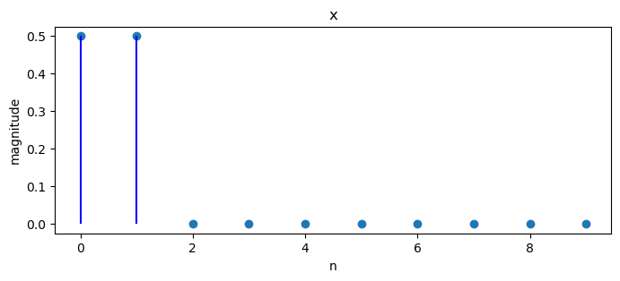
Consider the following example.

\begin{array}{r} x_{n} = {\begin{cases} 1 / 2 & n = 0, 1 \\ 0 & otherwise \end{cases} \end{array}

x = np.zeros(10)
x[0:2] = 1/2

array([0.5, 0.5, 0. , 0. , 0. , 0. , 0. , 0. , 0. , 0. ])

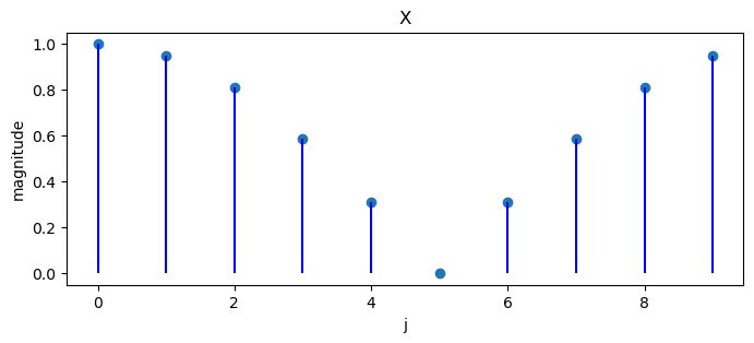
Apply a discrete Fourier transform.

X = DFT(x)

array([ 1.   +0.j   ,  0.905-0.294j,  0.655-0.476j,  0.345-0.476j,
        0.095-0.294j, -0.   +0.j   ,  0.095+0.294j,  0.345+0.476j,
        0.655+0.476j,  0.905+0.294j])

We can plot magnitudes of a sequence of numbers and the associated discrete Fourier transform.

def plot_magnitude(x=None, X=None):

    data = []
    names = []
    xs = []
    if (x is not None):
        data.append(x)
        names.append('x')
        xs.append('n')
    if (X is not None):
        data.append(X)
        names.append('X')
        xs.append('j')

    num = len(data)
    for i in range(num):
        n = data[i].size
        plt.figure(figsize=(8, 3))
        plt.scatter(range(n), np.abs(data[i]))
        plt.vlines(range(n), 0, np.abs(data[i]), color='b')

        plt.xlabel(xs[i])
        plt.ylabel('magnitude')
        plt.title(names[i])
        plt.show()

plot_magnitude(x=x, X=X)

_images/94c5fa8560aa85278fa163fa3d65e264d37efd5fe5add04304c4967a11e8f63f.png

_images/8d1f91c96975dbda17fa1356338fab26004669a223575f5f5d9a9f08ba19b165.png

The inverse Fourier transform transforms a Fourier transform $X$ of $x$ back to $x$ .

The inverse Fourier transform is defined as

x_{n} = \sum_{k = 0}^{N - 1} \frac{1}{N} X_{k} e^{2 π (\frac{k n}{N}) i}, n = 0, 1, \dots, N - 1

def inverse_transform(X):

    N = len(X)
    w = np.e ** (complex(0, 2*np.pi/N))

    x = np.zeros(N, dtype=complex)
    for n in range(N):
        for k in range(N):
            x[n] += X[k] * w ** (k * n) / N

    return x

inverse_transform(X)

array([ 0.5+0.j,  0.5-0.j, -0. -0.j, -0. -0.j, -0. -0.j, -0. -0.j,
       -0. +0.j, -0. +0.j, -0. +0.j, -0. +0.j])

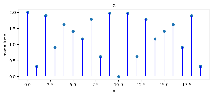
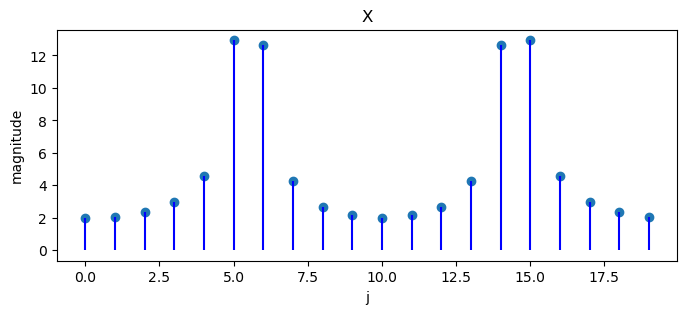
Another example is

x_{n} = 2 \cos (2 π \frac{11}{40} n), n = 0, 1, 2, \dots 19

Since $N = 20$ , we cannot use an integer multiple of $\frac{1}{20}$ to represent a frequency $\frac{11}{40}$ .

To handle this, we shall end up using all $N$ of the availble frequencies in the DFT.

Since $\frac{11}{40}$ is in between $\frac{10}{40}$ and $\frac{12}{40}$ (each of which is an integer multiple of $\frac{1}{20}$ ), the complex coefficients in the DFT have their largest magnitudes at $k = 5, 6, 15, 16$ , not just at a single frequency.

N = 20
x = np.empty(N)

for j in range(N):
    x[j] = 2 * np.cos(2 * np.pi * 11 * j / 40)

X = DFT(x)

plot_magnitude(x=x, X=X)

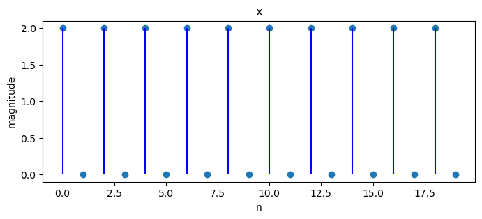
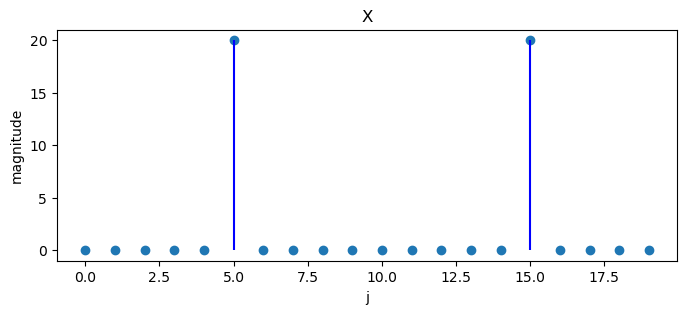
_images/fcecbaf03f711916b5c1fe21de2ba0ec188857042a6cc8d86a59aa74b01b1fbf.png

_images/2cd34536b42beebd90214400247115f391e384b3b95deea500fbadcd8fd8ad61.png

What happens if we change the last example to $x_{n} = 2 \cos (2 π \frac{10}{40} n)$ ?

Note that $\frac{10}{40}$ is an integer multiple of $\frac{1}{20}$ .

N = 20
x = np.empty(N)

for j in range(N):
    x[j] = 2 * np.cos(2 * np.pi * 10 * j / 40)

X = DFT(x)

plot_magnitude(x=x, X=X)

_images/660fbe197375132f5eb73d523205ecba334778976782cefa3031355a1359bbde.png

_images/d6bf89ca0aae5e41cb92357ab4dbcbcefb228df261524c4e4d00224c83053a1f.png

If we represent the discrete Fourier transform as a matrix, we discover that it equals the matrix $F_{N}$ of eigenvectors of the permutation matrix $P_{N}$ .

We can use the example where $x_{n} = 2 \cos (2 π \frac{11}{40} n), n = 0, 1, 2, \dots 19$ to illustrate this.

N = 20
x = np.empty(N)

for j in range(N):
    x[j] = 2 * np.cos(2 * np.pi * 11 * j / 40)

array([ 2.   , -0.313, -1.902,  0.908,  1.618, -1.414, -1.176,  1.782,
        0.618, -1.975, -0.   ,  1.975, -0.618, -1.782,  1.176,  1.414,
       -1.618, -0.908,  1.902,  0.313])

First use the summation formula to transform $x$ to $X$ .

X = DFT(x)
X

array([2. +0.j   , 2. +0.558j, 2. +1.218j, 2. +2.174j, 2. +4.087j,
       2.+12.785j, 2.-12.466j, 2. -3.751j, 2. -1.801j, 2. -0.778j,
       2. -0.j   , 2. +0.778j, 2. +1.801j, 2. +3.751j, 2.+12.466j,
       2.-12.785j, 2. -4.087j, 2. -2.174j, 2. -1.218j, 2. -0.558j])

Now let’s evaluate the outcome of postmultiplying the eigenvector matrix $F_{20}$ by the vector $x$ , a product that we claim should equal the Fourier tranform of the sequence ${x_{n}}_{n = 0}^{N - 1}$ .

F20, _ = construct_F(20)

F20 @ x

array([2. +0.j   , 2. +0.558j, 2. +1.218j, 2. +2.174j, 2. +4.087j,
       2.+12.785j, 2.-12.466j, 2. -3.751j, 2. -1.801j, 2. -0.778j,
       2. -0.j   , 2. +0.778j, 2. +1.801j, 2. +3.751j, 2.+12.466j,
       2.-12.785j, 2. -4.087j, 2. -2.174j, 2. -1.218j, 2. -0.558j])

Similarly, the inverse DFT can be expressed as a inverse DFT matrix $F_{20}^{- 1}$ .

F20_inv = np.linalg.inv(F20)
F20_inv @ X

array([ 2.   -0.j, -0.313-0.j, -1.902+0.j,  0.908-0.j,  1.618-0.j,
       -1.414+0.j, -1.176+0.j,  1.782+0.j,  0.618-0.j, -1.975-0.j,
       -0.   +0.j,  1.975-0.j, -0.618-0.j, -1.782+0.j,  1.176+0.j,
        1.414-0.j, -1.618-0.j, -0.908+0.j,  1.902+0.j,  0.313-0.j])