26. Incorrect Models#

26.1. Overview#

This is a sequel to this quantecon lecture.

We discuss two ways to create compound lottery and their consequences.

A compound lottery can be said to create a mixture distribution.

Our two ways of constructing a compound lottery will differ in their timing.

• in one, mixing between two possible probability distributions will occur once and all at the beginning of time

• in the other, mixing between the same two possible possible probability distributions will occur each period

The statistical setting is close but not identical to the problem studied in that quantecon lecture.

In that lecture, there were two i.i.d. processes that could possibly govern successive draws of a non-negative random variable $W$.

Nature decided once and for all whether to make a sequence of IID draws from either $f$ or from $g$.

That lecture studied an agent who knew both $f$ and $g$ but did not know which distribution nature chose at time $-1$.

The agent represented that ignorance by assuming that nature had chosen $f$ or $g$ by flipping an unfair coin that put probability ${\pi }_{-1}$ on probability distribution $f$.

That assumption allowed the agent to construct a subjective joint probability distribution over the random sequence $\{W_t{\}}_{t=0}^{\mathrm{\infty }}$.

We studied how the agent would then use the laws of conditional probability and an observed history $w^t=\{w_s{\}}_{t=0}^t$ to form

However, in the setting of this lecture, that rule imputes to the agent an incorrect model.

The reason is that now the wage sequence is actually described by a different statistical model.

Thus, we change the quantecon lecture specification in the following way.

Now, each period $t\ge 0$, nature flips a possibly unfair coin that comes up $f$ with probability $\alpha$ and $g$ with probability $1-\alpha$.

Thus, naturally perpetually draws from the mixture distribution with c.d.f.

We’ll study two agents who try to learn about the wage process, but who use different statistical models.

Both types of agent know $f$ and $g$ but neither knows $\alpha$.

Our first type of agent erroneously thinks that at time $-1$ nature once and for all chose $f$ or $g$ and thereafter permanently draws from that distribution.

Our second type of agent knows, correctly, that nature mixes $f$ and $g$ with mixing probability $\alpha \in (0,1)$ each period, though the agent doesn’t know the mixing parameter.

Our first type of agent applies the learning algorithm described in this quantecon lecture.

In the context of the statistical model that prevailed in that lecture, that was a good learning algorithm and it enabled the Bayesian learner eventually to learn the distribution that nature had drawn at time $-1$.

This is because the agent’s statistical model was correct in the sense of being aligned with the data generating process.

But in the present context, our type 1 decision maker’s model is incorrect because the model $h$ that actually generates the data is neither $f$ nor $g$ and so is beyond the support of the models that the agent thinks are possible.

Nevertheless, we’ll see that our first type of agent muddles through and eventually learns something interesting and useful, even though it is not true.

Instead, it turn out that our type 1 agent who is armed with a wrong statistical model ends up learning whichever probability distribution, $f$ or $g$, is in a special sense closest to the $h$ that actually generates the data.

We’ll tell the sense in which it is closest.

Our second type of agent understands that nature mixes between $f$ and $g$ each period with a fixed mixing probability $\alpha$.

But the agent doesn’t know $\alpha$.

The agent sets out to learn $\alpha$ using Bayes’ law applied to his model.

His model is correct in the sense that it includes the actual data generating process $h$ as a possible distribution.

In this lecture, we’ll learn about

• how nature can mix between two distributions $f$ and $g$ to create a new distribution $h$.

• The Kullback-Leibler statistical divergence https://en.wikipedia.org/wiki/Kullback–Leibler_divergence that governs statistical learning under an incorrect statistical model

• A useful Python function numpy.searchsorted that, in conjunction with a uniform random number generator, can be used to sample from an arbitrary distribution

As usual, we’ll start by importing some Python tools.

import matplotlib.pyplot as plt
plt.rcParams["figure.figsize"] = (11, 5)  #set default figure size
import numpy as np
from numba import vectorize, jit
from math import gamma
import pandas as pd
import scipy.stats as sp
from scipy.integrate import quad

import seaborn as sns
colors = sns.color_palette()

import numpyro
import numpyro.distributions as dist
from numpyro.infer import MCMC, NUTS

import jax.numpy as jnp
from jax import random

np.random.seed(142857)

@jit
def set_seed():
    np.random.seed(142857)
set_seed()

Let’s use Python to generate two beta distributions

# Parameters in the two beta distributions.
F_a, F_b = 1, 1
G_a, G_b = 3, 1.2

@vectorize
def p(x, a, b):
    r = gamma(a + b) / (gamma(a) * gamma(b))
    return r * x** (a-1) * (1 - x) ** (b-1)

# The two density functions.
f = jit(lambda x: p(x, F_a, F_b))
g = jit(lambda x: p(x, G_a, G_b))

@jit
def simulate(a, b, T=50, N=500):
    '''
    Generate N sets of T observations of the likelihood ratio,
    return as N x T matrix.

    '''

    l_arr = np.empty((N, T))

    for i in range(N):

        for j in range(T):
            w = np.random.beta(a, b)
            l_arr[i, j] = f(w) / g(w)

    return l_arr

We’ll also use the following Python code to prepare some informative simulations

l_arr_g = simulate(G_a, G_b, N=50000)
l_seq_g = np.cumprod(l_arr_g, axis=1)

l_arr_f = simulate(F_a, F_b, N=50000)
l_seq_f = np.cumprod(l_arr_f, axis=1)

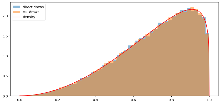
26.2. Sampling from Compound Lottery $H$#

We implement two methods to draw samples from our mixture model $\alpha F+(1-\alpha )G$.

We’ll generate samples using each of them and verify that they match well.

Here is pseudo code for a direct “method 1” for drawing from our compound lottery:

• Step one:

  • use the numpy.random.choice function to flip an unfair coin that selects distribution $F$ with prob $\alpha$ and $G$ with prob $1-\alpha$

• Step two:

  • draw from either $F$ or $G$, as determined by the coin flip.

• Step three:

  • put the first two steps in a big loop and do them for each realization of $w$

Our second method uses a uniform distribution and the following fact that we also described and used in the quantecon lecture https://python.quantecon.org/prob_matrix.html:

• If a random variable $X$ has c.d.f. $F(X)$, then a random variable $F^{-1}(U)$ also has c.d.f. $F(x)$, where $U$ is a uniform random variable on $[0,1]$.

In other words, if $X\sim F(x)$ we can generate a random sample from $F$ by drawing a random sample from a uniform distribution on $[0,1]$ and computing $F^{-1}(U)$.

We’ll use this fact in conjunction with the numpy.searchsorted command to sample from $H$ directly.

See https://numpy.org/doc/stable/reference/generated/numpy.searchsorted.html for the searchsorted function.

See the Mr. P Solver video on Monte Carlo simulation to see other applications of this powerful trick.

In the Python code below, we’ll use both of our methods and confirm that each of them does a good job of sampling from our target mixture distribution.

@jit
def draw_lottery(p, N):
    "Draw from the compound lottery directly."

    draws = []
    for i in range(0, N):
        if np.random.rand()<=p:
            draws.append(np.random.beta(F_a, F_b))
        else:
            draws.append(np.random.beta(G_a, G_b))

    return np.array(draws)

def draw_lottery_MC(p, N):
    "Draw from the compound lottery using the Monte Carlo trick."

    xs = np.linspace(1e-8,1-(1e-8),10000)
    CDF = p*sp.beta.cdf(xs, F_a, F_b) + (1-p)*sp.beta.cdf(xs, G_a, G_b)

    Us = np.random.rand(N)
    draws = xs[np.searchsorted(CDF[:-1], Us)]
    return draws

# verify
N = 100000
α = 0.0

sample1 = draw_lottery(α, N)
sample2 = draw_lottery_MC(α, N)

# plot draws and density function
plt.hist(sample1, 50, density=True, alpha=0.5, label='direct draws')
plt.hist(sample2, 50, density=True, alpha=0.5, label='MC draws')

xs = np.linspace(0,1,1000)
plt.plot(xs, α*f(xs)+(1-α)*g(xs), color='red', label='density')

plt.legend()
plt.show()

# %%timeit    # compare speed
# sample1 = draw_lottery(α, N=int(1e6))

# %%timeit
# sample2 = draw_lottery_MC(α, N=int(1e6))

Note: With numba acceleration the first method is actually only slightly slower than the second when we generated 1,000,000 samples.

26.3. Type 1 Agent#

We’ll now study what our type 1 agent learns

Remember that our type 1 agent uses the wrong statistical model, thinking that nature mixed between $f$ and $g$ once and for all at time $-1$.

The type 1 agent thus uses the learning algorithm studied in this quantecon lecture.

We’ll briefly review that learning algorithm now.

Let ${\pi }_t$ be a Bayesian posterior defined as

The likelihood ratio process plays a principal role in the formula that governs the evolution of the posterior probability ${\pi }_t$, an instance of Bayes’ Law.

Bayes’ law implies that $\{{\pi }_t\}$ obeys the recursion

with ${\pi }_0$ being a Bayesian prior probability that $q=f$, i.e., a personal or subjective belief about $q$ based on our having seen no data.

Below we define a Python function that updates belief $\pi$ using likelihood ratio $\ell$ according to recursion (26.1)

@jit
def update(π, l):
    "Update π using likelihood l"

    # Update belief
    π = π * l / (π * l + 1 - π)

    return π

Formula (26.1) can be generalized by iterating on it and thereby deriving an expression for the time $t$ posterior ${\pi }_{t+1}$ as a function of the time $0$ prior ${\pi }_0$ and the likelihood ratio process $L(w^{t+1})$ at time $t$.

To begin, notice that the updating rule

implies

Therefore

Since ${\pi }_0\in (0,1)$ and $L\left(w^{t+1}\right)>0$, we can verify that ${\pi }_{t+1}\in (0,1)$.

After rearranging the preceding equation, we can express ${\pi }_{t+1}$ as a function of $L\left(w^{t+1}\right)$, the likelihood ratio process at $t+1$, and the initial prior ${\pi }_0$

Formula (26.2) generalizes formula (26.1).

Formula (26.2) can be regarded as a one step revision of prior probability ${\pi }_0$ after seeing the batch of data ${\left\{w_i\right\}}_{i=1}^{t+1}$.

26.4. What a type 1 Agent Learns when Mixture $H$ Generates Data#

We now study what happens when the mixture distribution $h;\alpha$ truly generated the data each period.

A submartingale or supermartingale continues to describe ${\pi }_t$

It raises its ugly head and causes ${\pi }_t$ to converge either to $0$ or to $1$.

This is true even though in truth nature always mixes between $f$ and $g$.

After verifying that claim about possible limit points of ${\pi }_t$ sequences, we’ll drill down and study what fundamental force determines the limiting value of ${\pi }_t$.

Let’s set a value of $\alpha$ and then watch how ${\pi }_t$ evolves.

def simulate_mixed(α, T=50, N=500):
    """
    Generate N sets of T observations of the likelihood ratio,
    return as N x T matrix, when the true density is mixed h;α
    """

    w_s = draw_lottery(α, N*T).reshape(N, T)
    l_arr = f(w_s) / g(w_s)

    return l_arr

def plot_π_seq(α, π1=0.2, π2=0.8, T=200):
    """
    Compute and plot π_seq and the log likelihood ratio process
    when the mixed distribution governs the data.
    """

    l_arr_mixed = simulate_mixed(α, T=T, N=50)
    l_seq_mixed = np.cumprod(l_arr_mixed, axis=1)

    T = l_arr_mixed.shape[1]
    π_seq_mixed = np.empty((2, T+1))
    π_seq_mixed[:, 0] = π1, π2

    for t in range(T):
        for i in range(2):
            π_seq_mixed[i, t+1] = update(π_seq_mixed[i, t], l_arr_mixed[0, t])

    # plot
    fig, ax1 = plt.subplots()
    for i in range(2):
        ax1.plot(range(T+1), π_seq_mixed[i, :], label=rf"$\pi_0$={π_seq_mixed[i, 0]}")

    ax1.plot(np.nan, np.nan,  '--', color='b', label='Log likelihood ratio process')
    ax1.set_ylabel("$\pi_t$")
    ax1.set_xlabel("t")
    ax1.legend()
    ax1.set_title("when $\\alpha G + (1-\\alpha)$ F governs data")

    ax2 = ax1.twinx()
    ax2.plot(range(1, T+1), np.log(l_seq_mixed[0, :]), '--', color='b')
    ax2.set_ylabel("$log(L(w^{t}))$")

    plt.show()

<>:35: SyntaxWarning: invalid escape sequence '\p'
<>:35: SyntaxWarning: invalid escape sequence '\p'
/tmp/ipykernel_7565/2013898715.py:35: SyntaxWarning: invalid escape sequence '\p'
  ax1.set_ylabel("$\pi_t$")

plot_π_seq(α = 0.6)

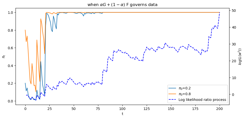
The above graph shows a sample path of the log likelihood ratio process as the blue dotted line, together with sample paths of ${\pi }_t$ that start from two distinct initial conditions.

Let’s see what happens when we change $\alpha$

plot_π_seq(α = 0.2)

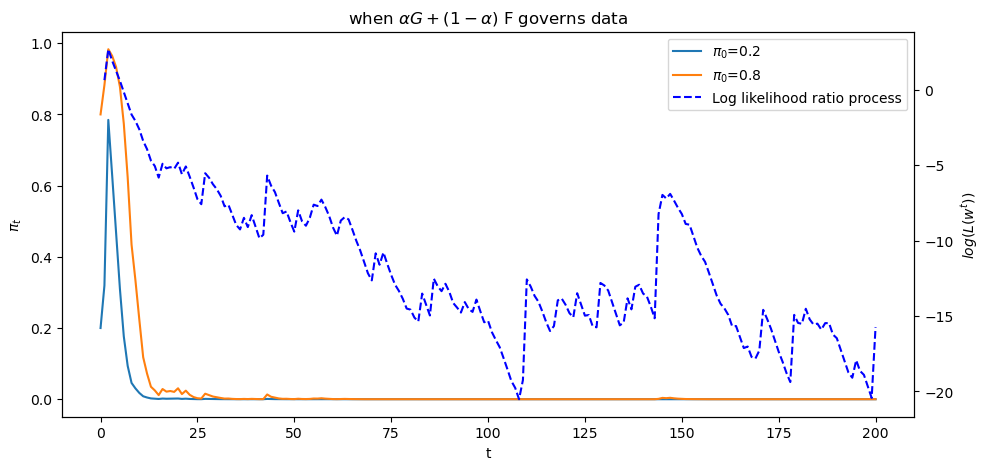
Evidently, $\alpha$ is having a big effect on the destination of ${\pi }_t$ as $t\to +\mathrm{\infty }$

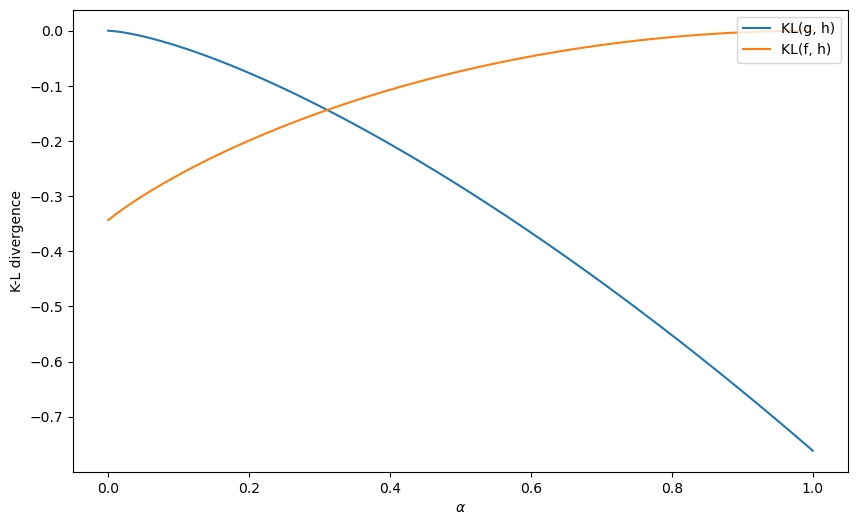
26.5. Kullback-Leibler Divergence Governs Limit of ${\pi }_t$#

To understand what determines whether the limit point of ${\pi }_t$ is $0$ or $1$ and how the answer depends on the true value of the mixing probability $\alpha \in (0,1)$ that generates

we shall compute the following two Kullback-Leibler divergences

and

We shall plot both of these functions against $\alpha$ as we use $\alpha$ to vary $h(w)=h(w|\alpha )$.

The limit of ${\pi }_t$ is determined by

The only possible limits are $0$ and $1$.

As $\to +\mathrm{\infty }$, ${\pi }_t$ goes to one if and only if $K{L}_f<K{L}_g$

@vectorize
def KL_g(α):
    "Compute the KL divergence between g and h."
    err = 1e-8                          # to avoid 0 at end points
    ws = np.linspace(err, 1-err, 10000)
    gs, fs = g(ws), f(ws)
    hs = α*fs + (1-α)*gs
    return np.sum(np.log(gs/hs)*hs)/10000

@vectorize
def KL_f(α):
    "Compute the KL divergence between f and h."
    err = 1e-8                          # to avoid 0 at end points
    ws = np.linspace(err, 1-err, 10000)
    gs, fs = g(ws), f(ws)
    hs = α*fs + (1-α)*gs
    return np.sum(np.log(fs/hs)*hs)/10000


# compute KL using quad in Scipy
def KL_g_quad(α):
    "Compute the KL divergence between g and h using scipy.integrate."
    h = lambda x: α*f(x) + (1-α)*g(x)
    return quad(lambda x: np.log(g(x)/h(x))*h(x), 0, 1)[0]

def KL_f_quad(α):
    "Compute the KL divergence between f and h using scipy.integrate."
    h = lambda x: α*f(x) + (1-α)*g(x)
    return quad(lambda x: np.log(f(x)/h(x))*h(x), 0, 1)[0]

# vectorize
KL_g_quad_v = np.vectorize(KL_g_quad)
KL_f_quad_v = np.vectorize(KL_f_quad)


# Let us find the limit point
def π_lim(α, T=5000, π_0=0.4):
    "Find limit of π sequence."
    π_seq = np.zeros(T+1)
    π_seq[0] = π_0
    l_arr = simulate_mixed(α, T, N=1)[0]

    for t in range(T):
        π_seq[t+1] = update(π_seq[t], l_arr[t])
    return π_seq[-1]

π_lim_v = np.vectorize(π_lim)

Let us first plot the KL divergences $K{L}_g\left(\alpha \right),K{L}_f\left(\alpha \right)$ for each $\alpha$.

α_arr = np.linspace(0, 1, 100)
KL_g_arr = KL_g(α_arr)
KL_f_arr = KL_f(α_arr)

fig, ax = plt.subplots(1, figsize=[10, 6])

ax.plot(α_arr, KL_g_arr, label='KL(g, h)')
ax.plot(α_arr, KL_f_arr, label='KL(f, h)')
ax.set_ylabel('K-L divergence')
ax.set_xlabel(r'$\alpha$')

ax.legend(loc='upper right')
plt.show()

# # using Scipy to compute KL divergence

# α_arr = np.linspace(0, 1, 100)
# KL_g_arr = KL_g_quad_v(α_arr)
# KL_f_arr = KL_f_quad_v(α_arr)

# fig, ax = plt.subplots(1, figsize=[10, 6])

# ax.plot(α_arr, KL_g_arr, label='KL(g, h)')
# ax.plot(α_arr, KL_f_arr, label='KL(f, h)')
# ax.set_ylabel('K-L divergence')

# ax.legend(loc='upper right')
# plt.show()

Let’s compute an $\alpha$ for which the KL divergence between $h$ and $g$ is the same as that between $h$ and $f$.

# where KL_f = KL_g
α_arr[np.argmin(np.abs(KL_g_arr-KL_f_arr))]

0.31313131313131315

We can compute and plot the convergence point ${\pi }_{\mathrm{\infty }}$ for each $\alpha$ to verify that the convergence is indeed governed by the KL divergence.

The blue circles show the limiting values of ${\pi }_t$ that simulations discover for different values of $\alpha$ recorded on the $x$ axis.

Thus, the graph below confirms how a minimum KL divergence governs what our type 1 agent eventually learns.

α_arr_x = α_arr[(α_arr<0.28)|(α_arr>0.38)]
π_lim_arr = π_lim_v(α_arr_x)

# plot
fig, ax = plt.subplots(1, figsize=[10, 6])

ax.plot(α_arr, KL_g_arr, label='KL(g, h)')
ax.plot(α_arr, KL_f_arr, label='KL(f, h)')
ax.set_ylabel('K-L divergence')
ax.set_xlabel(r'$\alpha$')

# plot KL
ax2 = ax.twinx()
# plot limit point
ax2.scatter(α_arr_x, π_lim_arr, facecolors='none', edgecolors='tab:blue', label=r'$\pi$ lim')
ax2.set_ylabel('π lim')

ax.legend(loc=[0.85, 0.8])
ax2.legend(loc=[0.85, 0.73])
plt.show()

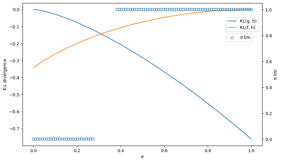
Evidently, our type 1 learner who applies Bayes’ law to his misspecified set of statistical models eventually learns an approximating model that is as close as possible to the true model, as measured by its Kullback-Leibler divergence.

26.6. Type 2 Agent#

We now describe how our type 2 agent formulates his learning problem and what he eventually learns.

Our type 2 agent understands the correct statistical model but acknowledges does not know $\alpha$.

We apply Bayes law to deduce an algorithm for learning $\alpha$ under the assumption that the agent knows that

but does not know $\alpha$.

We’ll assume that the person starts out with a prior probabilty ${\pi }_0(\alpha )$ on $\alpha \in (0,1)$ where the prior has one of the forms that we deployed in this quantecon lecture.

We’ll fire up numpyro and apply it to the present situation.

Bayes’ law now takes the form

We’ll use numpyro to approximate this equation.

We’ll create graphs of the posterior ${\pi }_t(\alpha )$ as $t\to +\mathrm{\infty }$ corresponding to ones presented in the quantecon lecture https://python.quantecon.org/bayes_nonconj.html.

We anticipate that a posterior distribution will collapse around the true $\alpha$ as $t\to +\mathrm{\infty }$.

Let us try a uniform prior first.

We use the Mixture class in Numpyro to construct the likelihood function.

α = 0.8

# simulate data with true α
data = draw_lottery(α, 1000)
sizes = [5, 20, 50, 200, 1000, 25000]

def model(w):
    α = numpyro.sample('α', dist.Uniform(low=0.0, high=1.0))

    y_samp = numpyro.sample('w',
        dist.Mixture(dist.Categorical(jnp.array([α, 1-α])), [dist.Beta(F_a, F_b), dist.Beta(G_a, G_b)]), obs=w)

def MCMC_run(ws):
    "Compute posterior using MCMC with observed ws"

    kernal = NUTS(model)
    mcmc = MCMC(kernal, num_samples=5000, num_warmup=1000, progress_bar=False)

    mcmc.run(rng_key=random.PRNGKey(142857), w=jnp.array(ws))
    sample = mcmc.get_samples()
    return sample['α']

The following code generates the graph below that displays Bayesian posteriors for $\alpha$ at various history lengths.

fig, ax = plt.subplots(figsize=(10, 6))

for i in range(len(sizes)):
    sample = MCMC_run(data[:sizes[i]])
    sns.histplot(
        data=sample, kde=True, stat='density', alpha=0.2, ax=ax,
        color=colors[i], binwidth=0.02, linewidth=0.05, label=f't={sizes[i]}'
    )
ax.set_title(r'$\pi_t(\alpha)$ as $t$ increases')
ax.legend()
ax.set_xlabel(r'$\alpha$')
plt.show()

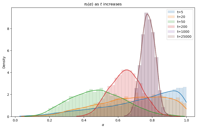
Evidently, the Bayesian posterior narrows in on the true value $\alpha =.8$ of the mixing parameter as the length of a history of observations grows.

26.7. Concluding Remarks#

Our type 1 person deploys an incorrect statistical model.

He believes that either $f$ or $g$ generated the $w$ process, but just doesn’t know which one.

That is wrong because nature is actually mixing each period with mixing probability $\alpha$.

Our type 1 agent eventually believes that either $f$ or $g$ generated the $w$ sequence, the outcome being determined by the model, either $f$ or $g$, whose KL divergence relative to $h$ is smaller.

Our type 2 agent has a different statistical model, one that is correctly specified.

He knows the parametric form of the statistical model but not the mixing parameter $\alpha$.

He knows that he does not know it.

But by using Bayes’ law in conjunction with his statistical model and a history of data, he eventually acquires a more and more accurate inference about $\alpha$.

This little laboratory exhibits some important general principles that govern outcomes of Bayesian learning of misspecified models.

Thus, the following situation prevails quite generally in empirical work.

A scientist approaches the data with a manifold $S$ of statistical models $s(X|\theta )$ , where $s$ is a probability distribution over a random vector $X$, $\theta \in \mathrm{\Theta }$ is a vector of parameters, and $\mathrm{\Theta }$ indexes the manifold of models.

The scientist with observations that he interprests as realizations $x$ of the random vector $X$ wants to solve an inverse problem of somehow inverting $s(x|\theta )$ to infer $\theta$ from $x$.

But the scientist’s model is misspecified, being only an approximation to an unknown model $h$ that nature uses to generate $X$.

If the scientist uses Bayes’ law or a related likelihood-based method to infer $\theta$, it occurs quite generally that for large sample sizes the inverse problem infers a $\theta$ that minimizes the KL divergence of the scientist’s model $s$ relative to nature’s model $h$.