23. A Bayesian Formulation of Friedman and Wald’s Problem#

23.1. Overview#

This lecture revisits the statistical decision problem presented to Milton Friedman and W. Allen Wallis during World War II when they were analysts at the U.S. Government’s Statistical Research Group at Columbia University.

In this lecture, we described how Abraham Wald [Wald, 1947] solved the problem by extending frequentist hypothesis testing techniques and formulating the problem sequentially.

As we learned in probability with matrices and two meanings of probability, a frequentist statistician views a probability distribution as measuring relative frequencies of a statistic that he anticipates constructing from a very long sequence of i.i.d. draws from a known probability distribution.

That known probability distribution is his ‘hypothesis’.

A frequentist statistician studies the distribution of that statistic under that known probability distribution

• when the distribution is a member of a set of parameterized probability distribution, his hypothesis takes the form of a particular parameter vector.

• this is what we mean when we say that the frequentist statistician ‘conditions on the parameters’

• he regards the parameters that are fixed numbers, known to nature, but not to him.

• the statistician copes with his ignorane of those parameters by constructing the type I and type II errors associated with frequentist hypothesis testing.

In this lecture, we reformulate Friedman and Wald’s problem by transforming our point of view from the ‘objective’ frequentist perspective of this lecture to an explicitly ‘subjective’ perspective taken by a Bayesian decision maker who regards parameters not as fixed numbers but as (hidden) random variables that are jointly distributed with the random variables that can be observed by sampling from that joint distribution.

To form that joint distribution, the Bayesian statistician supplements the conditional distributions used by the frequentist statistician with a prior probability distribution over the parameters that representive his personal, subjective opinion about those them.

To proceed in the way, we endow our decision maker with

• an initial prior subjective probability ${\pi }_{-1}\in (0,1)$ that nature uses to generate $\{z_k\}$ as a sequence of i.i.d. draws from $f_1$ rather than $f_0$.

• faith in Bayes’ law as a way to revise his subjective beliefs as observations on $\{z_k\}$ sequence arrive each period.

• a loss function that tells how the decision maker values type I and type II errors.

In our previous frequentist version, key ideas in play were:

• Type I and type II statistical errors

  • a type I error occurs when you reject a null hypothesis that is true

  • a type II error occurs when you accept a null hypothesis that is false

• Abraham Wald’s sequential probability ratio test

• The power of a statistical test

• The critical region of a statistical test

• A uniformly most powerful test

In this lecture about a Bayesian reformulation of the problem, additional ideas at work are

• an initial prior probability ${\pi }_{-1}$ that model $f_1$ generates the data

• Bayes’ Law

• a sequence of posterior probabilities that model $f_1$ is generating the data

• dynamic programming

This lecture uses ideas studied in this lecture, this lecture, and this lecture.

We’ll begin with some imports:

import numpy as np
import matplotlib.pyplot as plt
from numba import jit, prange, float64, int64
from numba.experimental import jitclass
from math import gamma

23.2. A Dynamic Programming Approach#

The following presentation of the problem closely follows Dmitri Berskekas’s treatment in Dynamic Programming and Stochastic Control [Bertsekas, 1975].

A decision-maker can observe a sequence of draws of a random variable $z$.

He (or she) wants to know which of two probability distributions $f_0$ or $f_1$ governs $z$.

Conditional on knowing that successive observations are drawn from distribution $f_0$, the sequence of random variables is independently and identically distributed (IID).

Conditional on knowing that successive observations are drawn from distribution $f_1$, the sequence of random variables is also independently and identically distributed (IID).

But the observer does not know which of the two distributions generated the sequence.

For reasons explained in Exchangeability and Bayesian Updating, this means that the sequence is not IID.

The observer has something to learn, namely, whether the observations are drawn from $f_0$ or from $f_1$.

The decision maker wants to decide which of the two distributions is generating outcomes.

We adopt a Bayesian formulation.

The decision maker begins with a prior probability

After observing $k+1$ observations $z_k,z_{k-1},\dots ,z_0$, he updates his personal probability that the observations are described by distribution $f_1$ to

which is calculated recursively by applying Bayes’ law:

After observing $z_k,z_{k-1},\dots ,z_0$, the decision-maker believes that $z_{k+1}$ has probability distribution

which is a mixture of distributions $f_0$ and $f_1$, with the weight on $f_1$ being the posterior probability that $f=f_1$ 1.

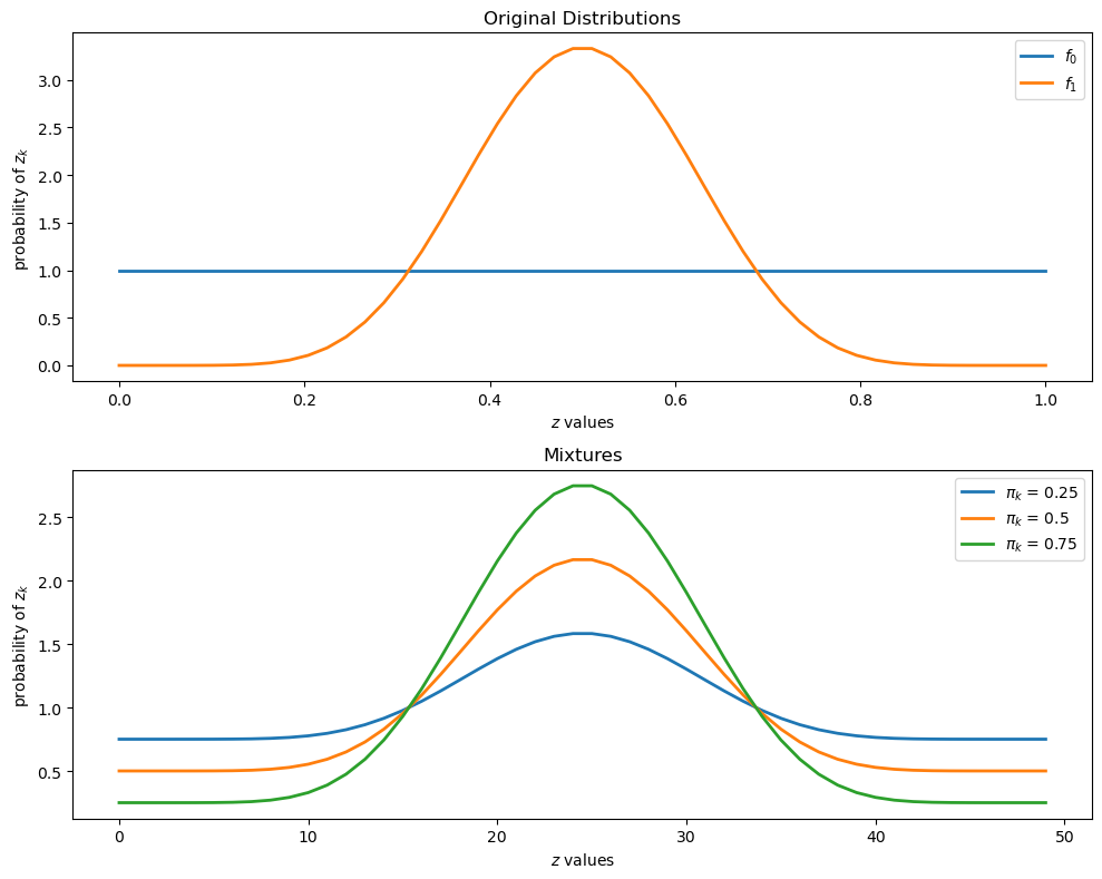
To illustrate such a distribution, let’s inspect some mixtures of beta distributions.

The density of a beta probability distribution with parameters $a$ and $b$ is

The next figure shows two beta distributions in the top panel.

The bottom panel presents mixtures of these distributions, with various mixing probabilities ${\pi }_k$

@jit
def p(x, a, b):
    r = gamma(a + b) / (gamma(a) * gamma(b))
    return r * x**(a-1) * (1 - x)**(b-1)

f0 = lambda x: p(x, 1, 1)
f1 = lambda x: p(x, 9, 9)
grid = np.linspace(0, 1, 50)

fig, axes = plt.subplots(2, figsize=(10, 8))

axes[0].set_title("Original Distributions")
axes[0].plot(grid, f0(grid), lw=2, label="$f_0$")
axes[0].plot(grid, f1(grid), lw=2, label="$f_1$")

axes[1].set_title("Mixtures")
for π in 0.25, 0.5, 0.75:
    y = (1 - π) * f0(grid) + π * f1(grid)
    axes[1].plot(y, lw=2, label=fr"$\pi_k$ = {π}")

for ax in axes:
    ax.legend()
    ax.set(xlabel="$z$ values", ylabel="probability of $z_k$")

plt.tight_layout()
plt.show()

23.2.3. Intuition#

Before proceeding, let’s try to guess what an optimal decision rule might look like.

Suppose at some given point in time that $\pi$ is close to 1.

Then our prior beliefs and the evidence so far point strongly to $f=f_1$.

If, on the other hand, $\pi$ is close to 0, then $f=f_0$ is strongly favored.

Finally, if $\pi$ is in the middle of the interval $[0,1]$, then we are confronted with more uncertainty.

This reasoning suggests a sequential decision rule that we illustrate in the following figure:

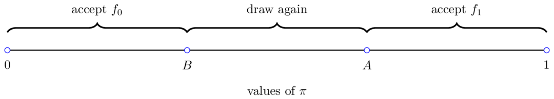
As we’ll see, this is indeed the correct form of the decision rule.

Our problem is to determine threshold values $A,B$ that somehow depend on the parameters described above.

You might like to pause at this point and try to predict the impact of a parameter such as $c$ or $L_0$ on $A$ or $B$.

23.3. Implementation#

First, we will construct a jitclass to store the parameters of the model

wf_data = [('a0', float64),          # Parameters of beta distributions
           ('b0', float64),
           ('a1', float64),
           ('b1', float64),
           ('c', float64),           # Cost of another draw
           ('π_grid_size', int64),
           ('L0', float64),          # Cost of selecting f0 when f1 is true
           ('L1', float64),          # Cost of selecting f1 when f0 is true
           ('π_grid', float64[:]),
           ('mc_size', int64),
           ('z0', float64[:]),
           ('z1', float64[:])]

@jitclass(wf_data)
class WaldFriedman:

    def __init__(self,
                 c=1.25,
                 a0=1,
                 b0=1,
                 a1=3,
                 b1=1.2,
                 L0=25,
                 L1=25,
                 π_grid_size=200,
                 mc_size=1000):

        self.a0, self.b0 = a0, b0
        self.a1, self.b1 = a1, b1
        self.c, self.π_grid_size = c, π_grid_size
        self.L0, self.L1 = L0, L1
        self.π_grid = np.linspace(0, 1, π_grid_size)
        self.mc_size = mc_size

        self.z0 = np.random.beta(a0, b0, mc_size)
        self.z1 = np.random.beta(a1, b1, mc_size)

    def f0(self, x):

        return p(x, self.a0, self.b0)

    def f1(self, x):

        return p(x, self.a1, self.b1)

    def f0_rvs(self):
        return np.random.beta(self.a0, self.b0)

    def f1_rvs(self):
        return np.random.beta(self.a1, self.b1)

    def κ(self, z, π):
        """
        Updates π using Bayes' rule and the current observation z
        """

        f0, f1 = self.f0, self.f1

        π_f0, π_f1 = (1 - π) * f0(z), π * f1(z)
        π_new = π_f1 / (π_f0 + π_f1)

        return π_new

As in the optimal growth lecture, to approximate a continuous value function

• We iterate at a finite grid of possible values of $\pi$.

• When we evaluate $\mathbb{E}[J({\pi }^{\prime })]$ between grid points, we use linear interpolation.

We define the operator function Q below.

@jit(nopython=True, parallel=True)
def Q(h, wf):

    c, π_grid = wf.c, wf.π_grid
    L0, L1 = wf.L0, wf.L1
    z0, z1 = wf.z0, wf.z1
    mc_size = wf.mc_size

    κ = wf.κ

    h_new = np.empty_like(π_grid)
    h_func = lambda p: np.interp(p, π_grid, h)

    for i in prange(len(π_grid)):
        π = π_grid[i]

        # Find the expected value of J by integrating over z
        integral_f0, integral_f1 = 0, 0
        for m in range(mc_size):
            π_0 = κ(z0[m], π)  # Draw z from f0 and update π
            integral_f0 += min(π_0 * L0, (1 - π_0) * L1, h_func(π_0))

            π_1 = κ(z1[m], π)  # Draw z from f1 and update π
            integral_f1 += min(π_1 * L0, (1 - π_1) * L1, h_func(π_1))

        integral = ((1 - π) * integral_f0 + π * integral_f1) / mc_size

        h_new[i] = c + integral

    return h_new

To solve the key functional equation, we will iterate using Q to find the fixed point

@jit
def solve_model(wf, tol=1e-4, max_iter=1000):
    """
    Compute the continuation cost function

    * wf is an instance of WaldFriedman
    """

    # Set up loop
    h = np.zeros(len(wf.π_grid))
    i = 0
    error = tol + 1

    while i < max_iter and error > tol:
        h_new = Q(h, wf)
        error = np.max(np.abs(h - h_new))
        i += 1
        h = h_new

    if error > tol:
        print("Failed to converge!")

    return h_new

23.4. Analysis#

Let’s inspect outcomes.

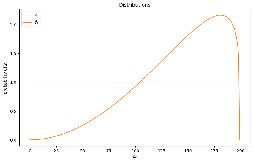
We will be using the default parameterization with distributions like so

wf = WaldFriedman()

fig, ax = plt.subplots(figsize=(10, 6))
ax.plot(wf.f0(wf.π_grid), label="$f_0$")
ax.plot(wf.f1(wf.π_grid), label="$f_1$")
ax.set(ylabel="probability of $z_k$", xlabel="$z_k$", title="Distributions")
ax.legend()

plt.show()

23.4.1. Cost Function#

To solve the model, we will call our solve_model function

h_star = solve_model(wf)    # Solve the model

We will also set up a function to compute the cutoffs $A$ and $B$ and plot these on our cost function plot

@jit
def find_cutoff_rule(wf, h):

    """
    This function takes a continuation cost function and returns the
    corresponding cutoffs of where you transition between continuing and
    choosing a specific model
    """

    π_grid = wf.π_grid
    L0, L1 = wf.L0, wf.L1

    # Evaluate cost at all points on grid for choosing a model
    cost_f0 = π_grid * L0
    cost_f1 = (1 - π_grid) * L1
    
    # Find B: largest π where cost_f0 <= min(cost_f1, h)
    optimal_cost = np.minimum(np.minimum(cost_f0, cost_f1), h)
    choose_f0 = (cost_f0 <= cost_f1) & (cost_f0 <= h)
    
    if np.any(choose_f0):
        B = π_grid[choose_f0][-1]  # Last point where we choose f0
    else:
        assert False, "No point where we choose f0"
    
    # Find A: smallest π where cost_f1 <= min(cost_f0, h)  
    choose_f1 = (cost_f1 <= cost_f0) & (cost_f1 <= h)
    
    if np.any(choose_f1):
        A = π_grid[choose_f1][0]  # First point where we choose f1
    else:
        assert False, "No point where we choose f1"

    return (B, A)

B, A = find_cutoff_rule(wf, h_star)
cost_L0 = wf.π_grid * wf.L0
cost_L1 = (1 - wf.π_grid) * wf.L1

fig, ax = plt.subplots(figsize=(10, 6))

ax.plot(wf.π_grid, h_star, label='sample again')
ax.plot(wf.π_grid, cost_L1, label='choose f1')
ax.plot(wf.π_grid, cost_L0, label='choose f0')
ax.plot(wf.π_grid,
        np.amin(np.column_stack([h_star, cost_L0, cost_L1]),axis=1),
        lw=15, alpha=0.1, color='b', label=r'$J(\pi)$')

ax.annotate(r"$B$", xy=(B + 0.01, 0.5), fontsize=14)
ax.annotate(r"$A$", xy=(A + 0.01, 0.5), fontsize=14)

plt.vlines(B, 0, (1 - B) * wf.L1, linestyle="--")
plt.vlines(A, 0, A * wf.L0, linestyle="--")

ax.set(xlim=(0, 1), ylim=(0, 0.5 * max(wf.L0, wf.L1)), ylabel="cost",
       xlabel=r"$\pi$", title=r"Cost function $J(\pi)$")

plt.legend(borderpad=1.1)
plt.show()

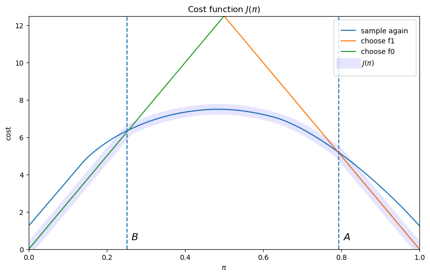
The cost function $J$ equals $\pi L_0$ for $\pi \le B$, and $(1-\pi )L_1$ for $\pi \ge A$.

The slopes of the two linear pieces of the cost function $J(\pi )$ are determined by $L_0$ and $-L_1$.

The cost function $J$ is smooth in the interior region, where the posterior probability assigned to $f_1$ is in the indecisive region $\pi \in (B,A)$.

The decision-maker continues to sample until the probability that he attaches to model $f_1$ falls below $B$ or above $A$.

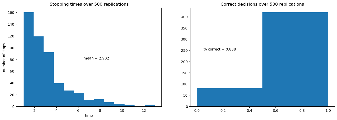
23.4.2. Simulations#

The next figure shows the outcomes of 500 simulations of the decision process.

On the left is a histogram of stopping times, i.e., the number of draws of $z_k$ required to make a decision.

The average number of draws is around 6.6.

On the right is the fraction of correct decisions at the stopping time.

In this case, the decision-maker is correct 80% of the time

def simulate(wf, true_dist, h_star, π_0=0.5):

    """
    This function takes an initial condition and simulates until it
    stops (when a decision is made)
    """

    f0, f1 = wf.f0, wf.f1
    f0_rvs, f1_rvs = wf.f0_rvs, wf.f1_rvs
    π_grid = wf.π_grid
    κ = wf.κ

    if true_dist == "f0":
        f, f_rvs = wf.f0, wf.f0_rvs
    elif true_dist == "f1":
        f, f_rvs = wf.f1, wf.f1_rvs

    # Find cutoffs
    B, A = find_cutoff_rule(wf, h_star)

    # Initialize a couple of useful variables
    decision_made = False
    π = π_0
    t = 0

    while decision_made is False:
        z = f_rvs()
        t = t + 1
        π = κ(z, π)
        if π < B:
            decision_made = True
            decision = 0
        elif π > A:
            decision_made = True
            decision = 1

    if true_dist == "f0":
        if decision == 0:
            correct = True
        else:
            correct = False

    elif true_dist == "f1":
        if decision == 1:
            correct = True
        else:
            correct = False

    return correct, π, t

def stopping_dist(wf, h_star, ndraws=250, true_dist="f0"):

    """
    Simulates repeatedly to get distributions of time needed to make a
    decision and how often they are correct
    """

    tdist = np.empty(ndraws, int)
    cdist = np.empty(ndraws, bool)

    for i in range(ndraws):
        correct, π, t = simulate(wf, true_dist, h_star)
        tdist[i] = t
        cdist[i] = correct

    return cdist, tdist

def simulation_plot(wf):
    h_star = solve_model(wf)
    ndraws = 500
    cdist, tdist = stopping_dist(wf, h_star, ndraws)

    fig, ax = plt.subplots(1, 2, figsize=(16, 5))

    ax[0].hist(tdist, bins=np.max(tdist))
    ax[0].set_title(f"Stopping times over {ndraws} replications")
    ax[0].set(xlabel="time", ylabel="number of stops")
    ax[0].annotate(f"mean = {np.mean(tdist)}", xy=(max(tdist) / 2,
                   max(np.histogram(tdist, bins=max(tdist))[0]) / 2))

    ax[1].hist(cdist.astype(int), bins=2)
    ax[1].set_title(f"Correct decisions over {ndraws} replications")
    ax[1].annotate(f"% correct = {np.mean(cdist)}",
                   xy=(0.05, ndraws / 2))

    plt.show()

simulation_plot(wf)

23.4.3. Comparative Statics#

Now let’s consider the following exercise.

We double the cost of drawing an additional observation.

Before you look, think about what will happen:

• Will the decision-maker be correct more or less often?

• Will he make decisions sooner or later?

wf = WaldFriedman(c=2.5)
simulation_plot(wf)

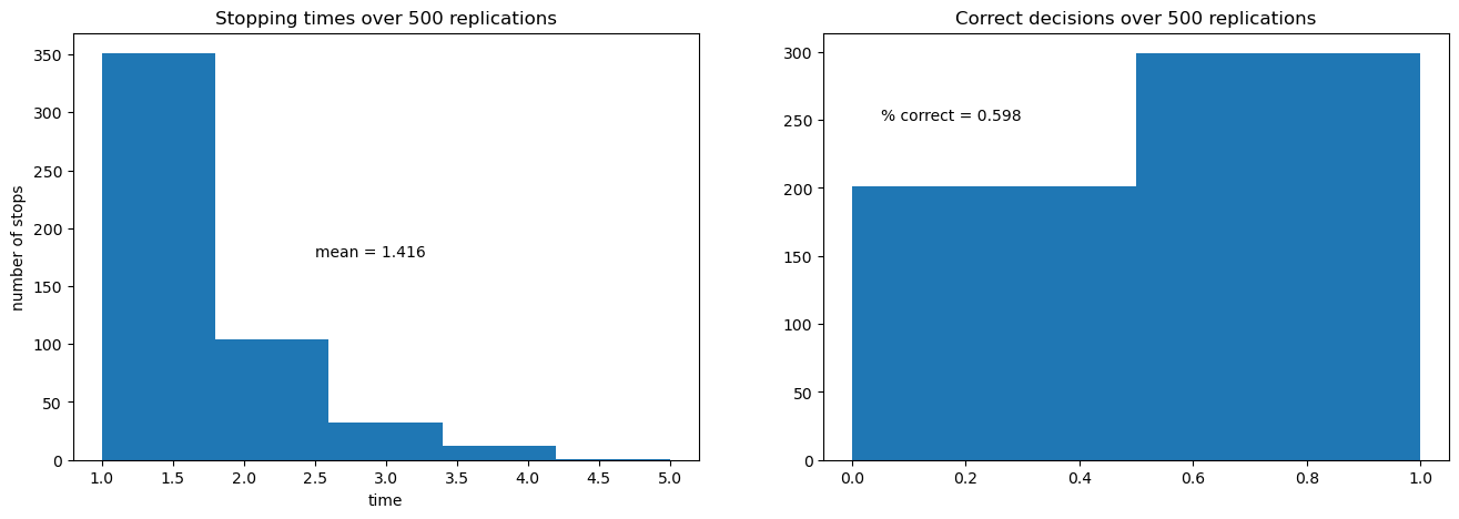
Increased cost per draw has induced the decision-maker to take fewer draws before deciding.

Because he decides with fewer draws, the percentage of time he is correct drops.

This leads to him having a higher expected loss when he puts equal weight on both models.

To facilitate comparative statics, we invite you to adjust the parameters of the model and investigate

• effects on the smoothness of the value function in the indecisive middle range as we increase the number of grid points in the piecewise linear approximation.

• effects of different settings for the cost parameters $L_0,L_1,c$, the parameters of two beta distributions $f_0$ and $f_1$, and the number of points and linear functions $m$ to use in the piece-wise continuous approximation to the value function.

• various simulations from $f_0$ and associated distributions of waiting times to making a decision.

• associated histograms of correct and incorrect decisions.

23.5. Related Lectures#

We’ll dig deeper into some of the ideas used here in the following lectures:

• this lecture discusses the key concept of exchangeability – a notion of conditional independences associated with foundations of statistical learning

• this lecture describes likelihood ratio processes and their role in frequentist and Bayesian statistical theories

• this lecture discusses the role of likelihood ratio processes in Bayesian learning

• this lecture returns to the subject of this lecture and studies whether the Captain’s hunch that the (frequentist) decision rule that the Navy had ordered him to use can be expected to be better or worse than our sequential decision rule

1

The decision maker acts as if he believes that the sequence of random variables $[z_0,z_1,\dots ]$ is exchangeable. See Exchangeability and Bayesian Updating and [Kreps, 1988] chapter 11, for discussions of exchangeability.